TextDeformer Paper

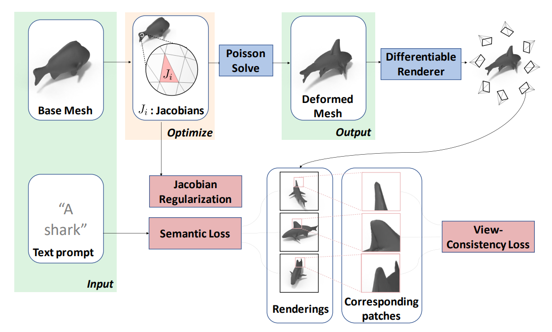
Overview of the Process

Given Pre-triangle Jacobians (Identity Initialized)
1. Jacobian Regularization loss
Compute deformed mesh by solving Poisson Equation
Render though differentiable renderer
Passing render image to CLIP
1. View Consistency loss
2. Semantic loss

Jacobians Described Transform and Poisson Equation

for a vector function $\vec{f}(u,v)$, the Jacobian is defined as $J = \vec{f}(u,v) \nabla^{T}_{uv} = \begin{bmatrix} \partial f_x/\partial u & \partial f_x/\partial v\\ \partial f_y/\partial u & \partial f_y/\partial v\\ \partial f_z/\partial u & \partial f_z/\partial v\\ \end{bmatrix}$

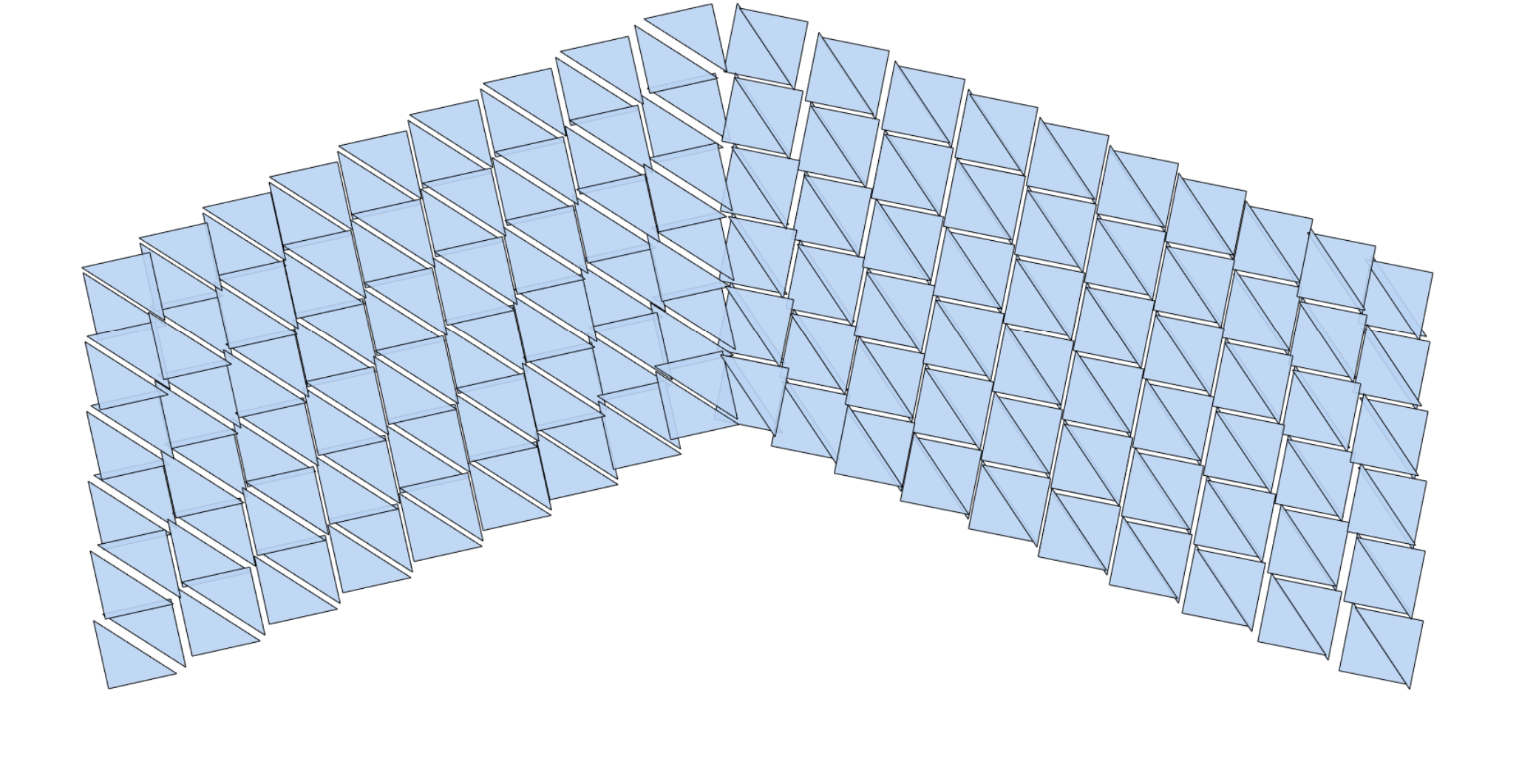
Jacobians describe the local linear transform of the non-linear transform

Jacobians separately transform Every Triangle, and is the source parameters for optimization

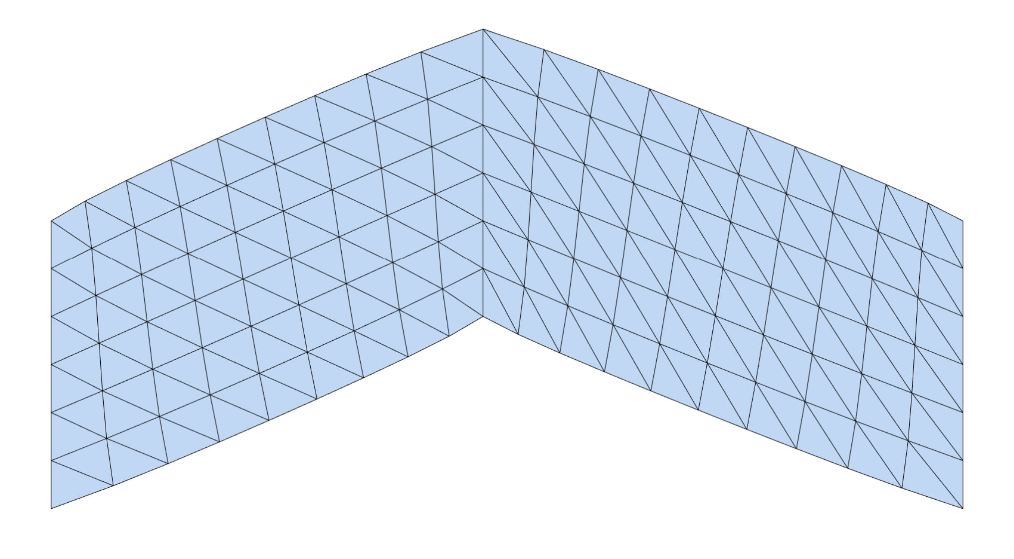
Solving Poisson Equation to restrict the mapping

$\Phi$ is the transform described by vertex offset

the minimum target is

\[\Phi^* = \min_{\phi}\sum_{f_i\in F} |f_i|\| \nabla_i(\Phi)-J_i \|_2^2\]

the $

f_i

$ is the area of the triangle, which is the weight term

$| \nabla_i(\Phi)-J_i |_2^2$ describes the match between pre-vertex transform and pre pre-triangle transform

this can be compute by solving the poisson equation

the predicting pre-triangle transform comes from

Neural Jacobian Fields: Learning Intrinsic Mappings of Arbitrary Meshes

which first given the predicting pre-triangle transform prediction then solving restriction to generate an acceptable mapping

in the Text Deformer author simplify this using only the pre-triangle transform (Jacobian) as the optimization parameter

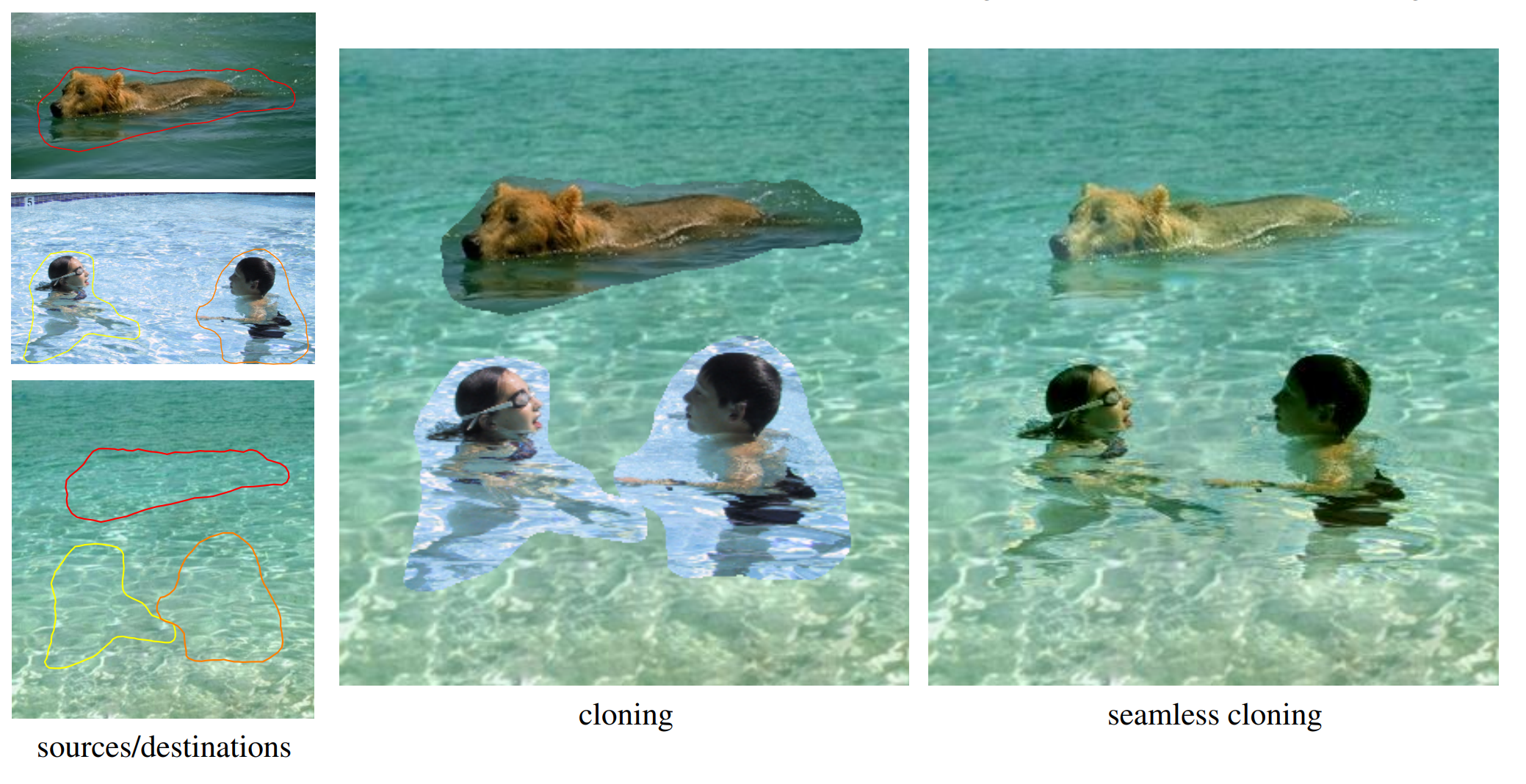
The poisson method is firstly being used in

Poisson Image Editing (SIGGRAPH 2004)

the goal is to minimize

\[\min_f \iint_{\Omega} \|\nabla f - v\|^2 \quad with \quad f|_{\partial \Omega} = f^*|_{\partial \Omega}\]

this yields the poisson equation

\[\Delta f = \nabla \cdot v \quad over \quad \Omega \quad with \quad f|_{\partial \Omega} = f^*|_{\partial \Omega}\]

to solve this equation, we need to encode the pixel value into a vector

to be specific $f$ is a $n \times c$ matrix, where $n$ is the number of pixel to be solved and $c$ is the number of channel

the discrete Laplacian operator on image is a convolution kernel

\[\begin{bmatrix} 0 & 1 & 0\\ 1 & -4 & 1\\ 0 & 1 & 0 \end{bmatrix}\]

and can be encode into a matrix $L$ which is a $n \times n$ matrix that

\[L_{ij} = \begin{cases} -4 & i = j\\ 1 & i \in N(j)\\ 0 & otherwise \end{cases}\] \[(L)_{1} = \begin{bmatrix} -4 & ... & 1 & ...& 1 & ...& 1 &...& 1 & ... \\ \end{bmatrix}\]

thus the poisson equation can be sovled as a linear system

\[L f = \nabla \cdot v\]

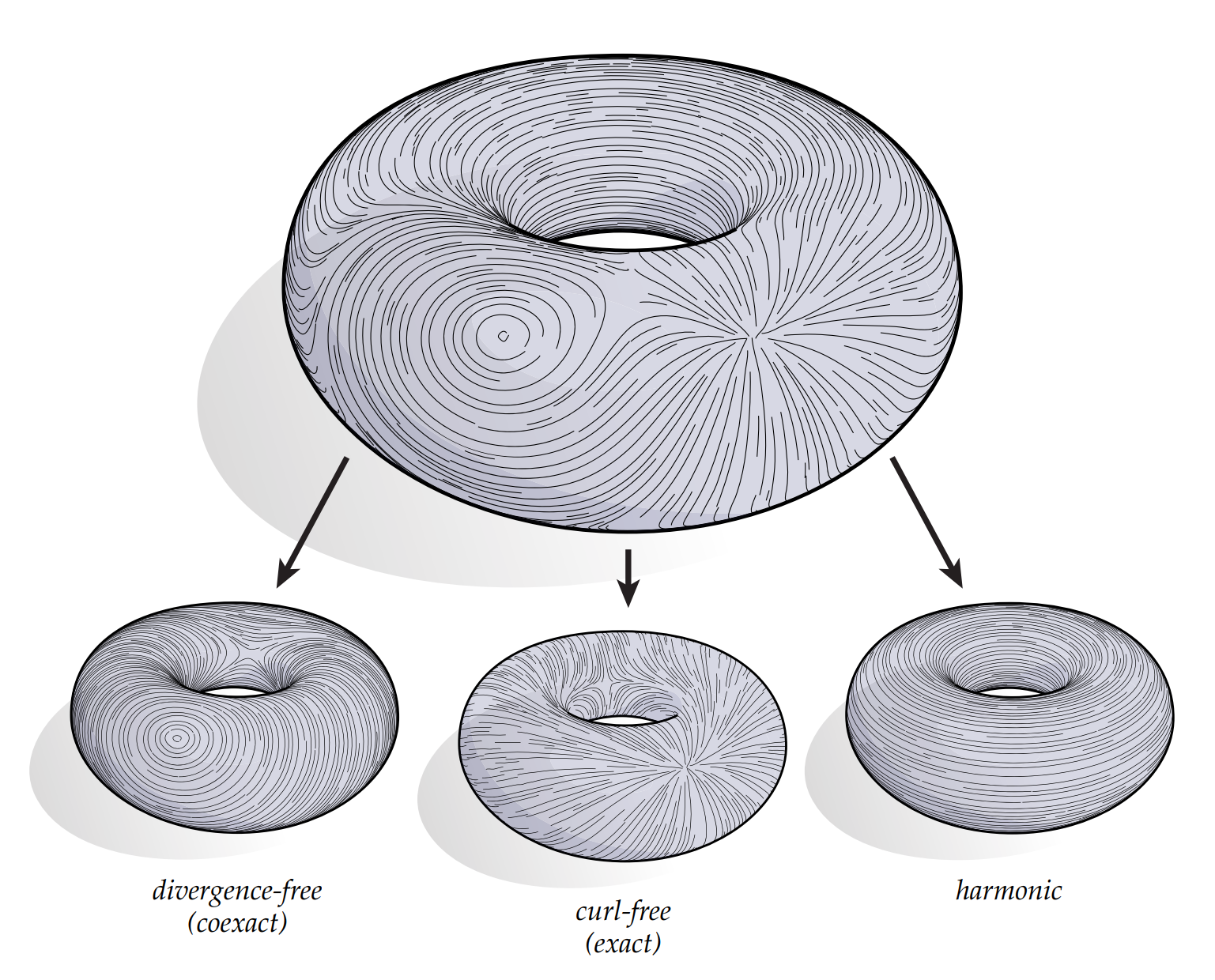
Mesh Editing with Poisson-Based Gradient Field Manipulation (Siggraph 2004) The Poisson equation is closely related to Helmholtz-Hodge vector field decomposition [Abrahamet al. 1988] which uniquely exists for a smooth 3D vector field wdefined in a region Ω:
\[\textbf{w} = \nabla \phi + \nabla \times v + \textbf{h}\]
The scalar potential field φ from this decomposition happens to be the solution of the following least-squares minimization
\[\min_{\phi} \iint_{\Omega} \|\nabla \phi - w\|^2 dA\]
whose solution can also be obtained by solving a Poisson equation,
\[\Delta \phi = \nabla \cdot w\]

Helmholtz-Hodge Decomposition from Discrete Differential Geometry: An Applied Introduction

least-squares minimization can be explained as finding a the potential field $\phi$ that minimize the difference between the gradient of $\phi$ (which is curl-free) and the vector field $w$, thus minimize the curl-free part of $w$, yielding a curl-free vector field

this is same as solving the Poisson equation which is obtained by diverging the vector field $w$ to cancel out the $\nabla \times v $ and $ \textbf{h}$ term

Solving Poisson Equation On Mesh

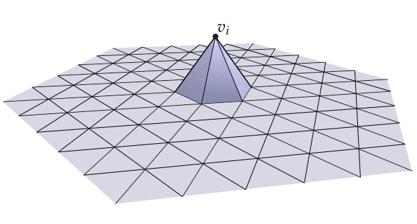
the discrete function on mesh is the sum of weighted basis function $\phi_i$ at each vertex $i$

the basis function $\phi_i$ is show as below, which is a hat function that value 1 at vertex $i$ and 0 at other vertex

thus a discrete function $f$ can be written as

\[f = \sum_{i=1}^n f_i \phi_i\]

the concept of point-wise and piece-wise:

point-wise: the function value is defined at every point
piece-wise: the function value is defined at every piece(triangle)

next we need to talk about the gradient on mesh

as the basis function is a hat function, the gradient of the basis function is a constant vector, thus the gradient operator is a linear operator that transform point-wise function to piece-wise function

the gradient operator is defined as

$\nabla f = \sum_{i=1}^n f_i \nabla \phi_i = G f$ $n$ is the number of vertex and $m$ is the number of triangle assume that $f$ is a scalar function, the f is a $n \times 1$ vector , $G$ is a $mk \times n$ matrix, it transform a point-wise scalar function to a piece-wise vector

to help understand tensor multiplication of $G$ we can view G as a $m \times n$ whitch contains $1 \times k$ matrix, the outer scope of the matrix compute in right to left order and the inner scope of the matrix compute in left to right order

\[G = \begin{bmatrix} \\ \begin{bmatrix} ... & ... \\ \end{bmatrix}_{1 \times k}\\ \\ \end{bmatrix}_{m \times n}\]

if $f$ is a vector function, then we have

\[Gf = \begin{bmatrix} \\ \begin{bmatrix} ... & ...\\ \end{bmatrix}_{1 \times k}\\ \\ \end{bmatrix}_{m \times n} \begin{bmatrix} \\ \begin{bmatrix} ... \\ ... \\ ...\\ \end{bmatrix}_{v \times 1}\\ \\ \end{bmatrix}_{n \times 1} = \begin{bmatrix} \\ \begin{bmatrix} ... & ... \\ ... & ... \\ ... & ... \\ \end{bmatrix}_{v \times k}\\ \\ \end{bmatrix}_{m \times 1}\]

standard poisson equation is defined as

\[\Delta u = f\]

to sovle u we express u as a linear combination of basis function

\[u = \sum_{i=1}^n x_i \phi_i\]

the inner product

\[<u,v> = \sum_{i=1}^n u_i v_i\]

and for function

\[<u,v> = \int_{\Omega} u v dA\]

to solve the poisson equation, we need to find a function $u$ that satisfy

\[<\Delta u - f, \phi_j> = 0\]

which means the difference between the Laplacian of $u$ and $f$ is orthogonal to all basis function $\phi_j$, thus minimizing the difference between the Laplacian of $u$ and $f$

this can be written as

\[<\Delta u, \phi_j> = <f, \phi_j>\]

for left side, we have

\[\begin{align*} <\Delta u, \phi_j> &= -<\nabla u, \nabla \phi_j>\\ &= -<\nabla (\sum_{i} x_i \phi_i), \nabla \phi_j>\\ &= -\sum_{i} x_i< \nabla \phi_i, \nabla \phi_j>\\ \end{align*}\]

define

\[L_{ij} =- < \nabla \phi_i, \nabla \phi_j>\]

then

\[<\Delta u, \phi_j> = L\vec{x}\]

cotan-Laplace operator

in short, the cotan-Laplace is

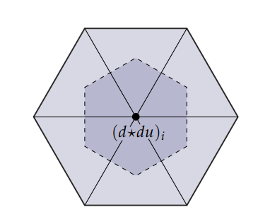
\[<\Delta u_i, \phi_j> = \frac{1}{2} \sum_{j \in N(i)} (\cot \alpha_{i} + \cot \beta_{i}) (u_j-u_i)\] \[L_{ij} = \begin{cases} -\frac{1}{2}\sum_{j \in N(i)} (\cot \alpha_{i} + \cot \beta_{i}) & i = j\\ \frac{1}{2}\cot \alpha_{i} + \cot \beta_{i} & i \in N(j)\\ 0 & otherwise \end{cases}\]

for right side, we have

\[\begin{align*} <f, \phi_j> &= <\sum_i b_i \phi_i, \phi_j>\\ &= \sum_i b_i <\phi_i, \phi_j> \end{align*}\] \[A_{ij}= <\phi_i, \phi_j>\] \[<f, \phi_j> = M\vec{b}\]

$M$ is called the mass matrix, which is a $n \times n$ diagonal matrix

\[M_{ii} = Area(v_i)\]

and finally we can solve the poisson equation by solving the linear system

\[L\vec{x} = M\vec{b}\]

also express as

\[M^{-1}Lu = f\]

this is Laplace-Beltrami(Cotan) Formula

we usually call $M^{-1}L$ as the discrete Laplace-Beltrami operator

the alternative way to compute L is using

\[L = G^T T G\]

where $T$ is the per-triangle area matrix or piece-wise mass matrix

to be intuitively understood this we first consider the scaler case

\[\begin{align*} \Delta \phi &= \nabla \cdot \nabla \phi\\ &= \begin{bmatrix}\frac{\partial}{\partial x}& \frac{\partial}{\partial y}& \frac{\partial}{\partial z}\end{bmatrix} \begin{bmatrix} \frac{\partial}{\partial x}\\ \frac{\partial}{\partial y}\\ \frac{\partial}{\partial z}\\ \end{bmatrix} \phi\\ &= \nabla^{T} \nabla \phi \end{align*}\]

the G first transform the point-wise function to piece-wise function the $T$ compute the area of each triangle the $G^T$ transform the piece-wise function to point-wise function

\[G = \begin{bmatrix} \\ \begin{bmatrix} ... & ... \\ \end{bmatrix}_{1 \times k}\\ \\ \end{bmatrix}_{m \times n}\qquad G^T = \begin{bmatrix} \\ \begin{bmatrix} ... \\ ... \\ \end{bmatrix}_{1 \times k}\\ \\ \end{bmatrix}_{n \times m}\]

as Laplace-Beltrami operator is $M^{-1}L$ bring $L$ into this $M^{-1}L = M^{-1}G^T T G$

we can assume that that point-wise mass matrix $M$ and piece-wise mass matrix $T$ cancel out each other leaving only the $G^T G$ which can be view as a $\Delta$

of curse this is only a intuitive explanation, keep in mind that $M^{-1}L$ is the correct way to compute the Laplace-Beltrami operator

\[G^T G \neq M^{-1}L\]

back to the original problemm we need to solve

\[\Phi^* = \min_{\phi}\sum_{f_i\in F} |f_i|\| \Phi\nabla_{i}^{T}-J_i \|_2^2\]

first convert this into poisson equation

\[\Delta \Phi = \nabla \cdot J\]

then using our tool we have

\[M^{-1}L\Phi = G^T J\]

computing $L$ can be accelerated by using

\[L = G^T T G\]

the mesh vertex transform $\Phi$ can be solved by

\[\Phi = L^{-1}MG^T J\]

the $J$ is our source parameter

by passing J through $L^{-1}MG^T$ we can get the vertex transform $\Phi$

$L^{-1}MG^T$ can be view as a Linear Layer in the network which is easy to compute the gradient

Jacobian Regularization loss

\[\mathcal{L}_{I}\left(t_{j}\right)=\alpha \sum_{i=1}^{|\mathcal{F}|}\left\|J_{i}-I\right\|_{2}\]

Differential Rendering

Modular Primitives for High-Performance Differentiable Rendering (NVIDIA)

Deferred Shading

Compute derivatives in the render pipeline for backward pass

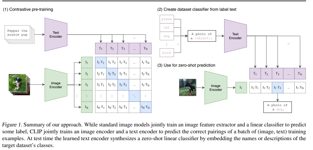
CLIP

Learning Transferable Visual Models From Natural Language Supervision

Pre-trained on large scale image-text dataset by OpenAI

View Consistency Loss

\[\mathcal{L}_{\mathrm{VC}}(v)=\sum_{i=1}^{|\mathcal{R}(\mathcal{M})||\mathcal{R}(\mathcal{M})|} \sum_{\substack{j=1 \\ j \neq i}} \operatorname{sim}\left(\mathcal{T}_{k}\left(P\left(v, r_{i}\right)\right), \mathcal{T}_{k}\left(P\left(v, r_{j}\right)\right)\right)\]

$v$ : vertex
$r$ : render
$\mathcal{R}(\mathcal{M})$ : all renders of mesh $\mathcal{M}$
$\mathcal{T}$ : transformer encoder blocks
$P$ : non-overlapping patches
$P\left(v, r\right)$ : nearest corresponding patch center of pixel $p\left(v, r\right)$ in $r$ that contains $v$

encourage vertices to have similar deep features across renders from different viewpoints

\[\mathcal{L}_{\mathrm{VC}}(M)= \beta \sum_{v \in \mathcal{V}} \mathcal{L}_{\mathrm{VC}}(v)\]

$\mathcal{V}$ : all vertices of mesh $\mathcal{M}$
$\beta$ : hyperparameter

Semantic Loss

\[\mathcal{L}_{\mathcal{P}}(\Phi^{*}, \mathcal{M}, \mathcal{P})=\operatorname{sim}(\operatorname{CLIP}(\Phi^{*}(\mathcal{M})), \operatorname{CLIP}(\mathcal{P}))\]

incorporating relative directions in CLIP’s embedding space can give stronger signals when the ptimization landscape between Φ∗ and P is unclear

\[\mathcal{L}_{\Delta \mathcal{P}}\left(\Phi^{*}, \mathcal{P}, \mathcal{P}_{0}\right)=\operatorname{sim}\left(\Delta \operatorname{CLIP}\left(\mathcal{P}, \mathcal{P}_{0}\right), \Delta \operatorname{CLIP}\left(\Phi^{*}(\mathcal{M}), \mathcal{M}\right)\right)\] \[\Delta \operatorname{CLIP}(\mathcal{P}, \mathcal{P}_{0})=\operatorname{CLIP}(\mathcal{P})-\operatorname{CLIP}\left(\mathcal{P}_{0}\right)\]

this enhance the semantic loss by comparing the difference between the prompt and the deformed mesh with the difference between the original mesh and the deformed mesh

$\mathcal{P}_0$ : prompt that discribes the original mesh
$\mathcal{P}$ : prompt that discribes the deformed mesh
$\mathcal{M}$ : original mesh
$\Phi^*(\mathcal{M})$ : deformed mesh
$\operatorname{CLIP}(\mathcal{P})$ : CLIP embedding of prompt $\mathcal{P}$
$\operatorname{CLIP}(\mathcal{M})$ : CLIP embedding of image rendered by differentiable renderer from mesh $\mathcal{M}$

TextDeformer Paper